Modelling the Spread of COVID-19
(27 March 2020)
A guide for Teachers
This page is not about current research controversies or public policy. It’s about teaching, and increasing the general public’s understanding of modelling.
All of us, around the world, are sequestered at home right now due to the predictions of a mathematical model, developed by a group at Imperial College London. The model predicts disaster, with deaths in the millions, unless population densities are greatly reduced by social distancing. Their primary paper was dated 16th March. The model they employed is based on their earlier paper. The supplement that gives the actual model is here.
The 16th March paper draws some harsh conclusions.
“For an uncontrolled epidemic, we predict critical care bed capacity would be exceeded as early as the second week in April, with an eventual peak in ICU or critical care bed demand that is over 30 times greater than the maximum supply in both countries.”
“We therefore conclude that epidemic suppression is the only viable strategy at the current time. The social and economic effects of the measures which are needed to achieve this policy goal will be profound.”
Their model is an agent-based model. That is, it postulates a large number of individuals moving around in space and encountering each other. The agent-based model (also called an individual-based model) allows them to do things like not assume a constant infectiousness parameter, but to have infectiousness vary from person to person (Individual infectiousness is assumed to be variable, described by a gamma distribution with mean 1 and shape parameter = 0.25
)
Notes for Teachers
There is some healthy controversy over the assumptions of this model, although all seem convinced that some kind of radical social distancing is required. This is not the place to enter that controversy. Follow the news sections of Nature and Science for updates. For example:
What the cruise-ship outbreaks reveal about COVID-19
It is not possible for even well-educated people to casually follow the details of the Imperial College Model. The reader would have to have an opinion on whether infectiousness is truly ‘described by a gamma distribution with mean 1 and shape parameter = 0.25’ Their paper is written for experts in epidemiological modeling, as it should be.
For Teachers You can help students get a feel for agent-based modeling, which is a widely-used modeling style.
Agent Based Modelling
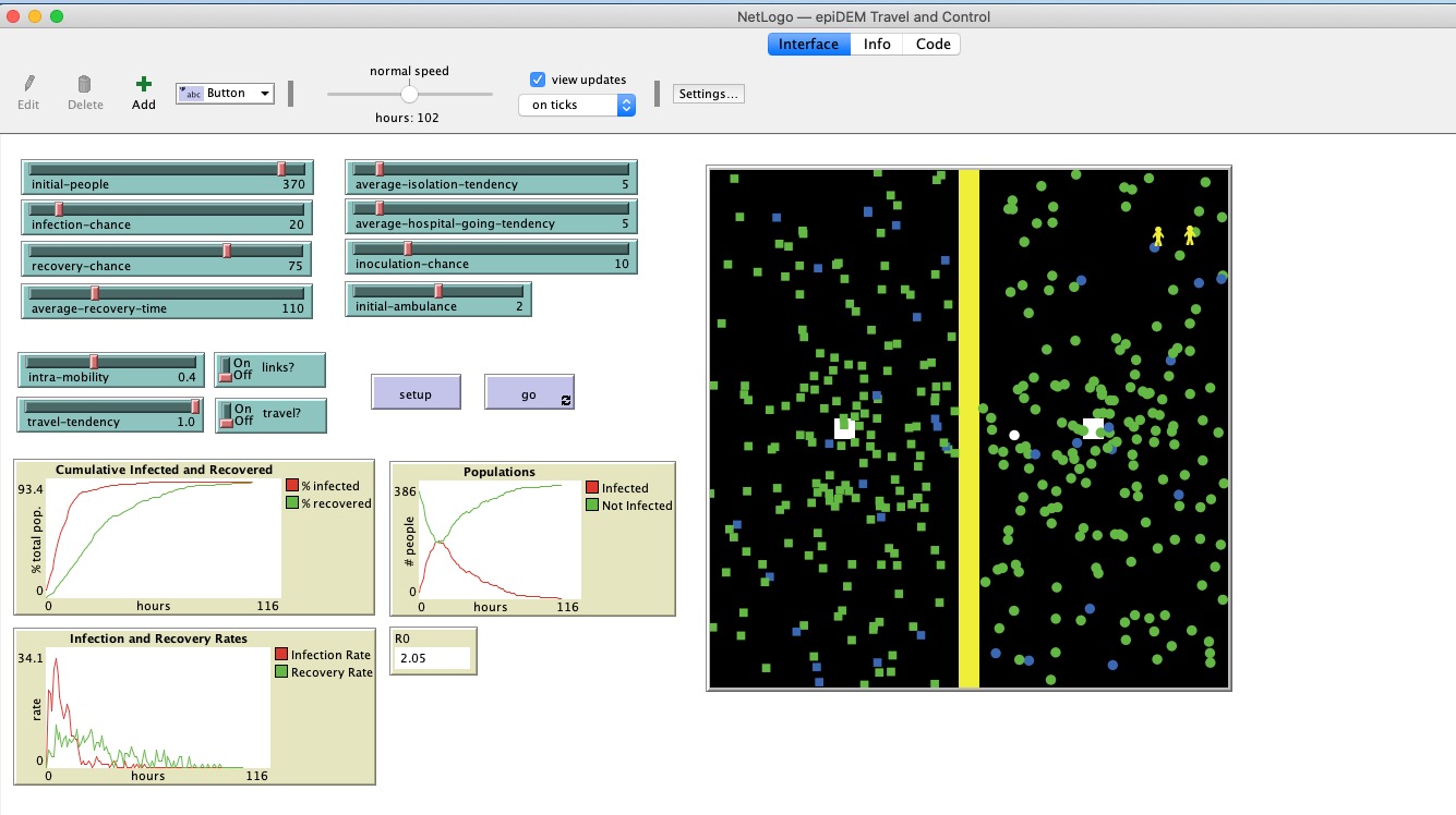
The best introduction to agent-based modeling is the free program NetLogo. Their model “epiDEM Travel and Control” gives you an instant model, that can be experimented with by computer-naive students within minutes of download. Students can manipulate parameters like ‘average recovery time’ and ‘average isolation tendency’, and watch what happens as the agents encounter each other.
Differential Equations Modelling
The other kind of modelling that is widely used is differential equations. Differential equation models differ from agent-based models. They don’t try to follow indivduals around, rather, they postulate overall or average quantities like “number of Susceptibles S”, “number of Infected I”, and “number of Recovered R”. (They are often referred to as “SIR” models). Then, we ask ‘what changes S?’, ‘what changes I?’ and ‘what changes R?’ and we see what consequences follow from the assumptions we have made.
Differential equations enable us to understand mechanisms more clearly than do agent-based models, because they can be studied mathematically. Also, agent-based models can sometimes be summarized as differential equation. For example, the diffusion partial differential equation is a high-level summary of the behavior of thousands of little random walker agents.
For simple differential equation models of the spread of an epidemic, most efforts build on the Anderson-May model of the spread of HIV 1. Here’s a version of their HIV transmission model from our text Modeling Life (Springer 2017, available free from Springer).
The video below explains SIR modeling in general and derives the Anderson-May model, and goes on to discuss a more recent model that was used by the US Centers for Disease Control to model control strategies for the Ebola outbreak in Africa in 2014. The video assumes that the viewer is familiar with population modelling using differential equations, such as the Predator/Prey model. (In the thumbnail portrait below, the instructor is pointing to the ‘social distancing’ parameter in the model.)
A runnable model
We created a runnable model of a COVID-19 type epidemic. We stress that this is a teaching tool, not a research tool. Students can adjust each of the parameters and see the outcomes.
In this particular model, there is no death, whether normal or disease related. That means it is not suitable for long-term modelling, or any situation in which death is a factor. The model will always go to an equilibrium where everyone has recovered and no one is infected. But the important thing is to follow the transient trajectory. Note that, with the default parameters here, 20% of the population will be medically symptomatic, needing medical attention, around day 30. This would drastically overwhelm available medical facilties.
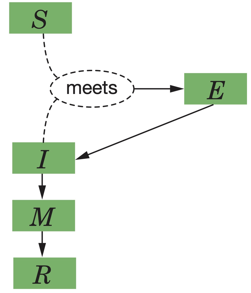
| State Variable | Short Description | Definition |
|---|---|---|
| \( S \) | Susceptibles | # of Susceptibles |
| \( E \) | Exposed | # of Exposed (infected but not yet infectious) |
| \( I \) | Infectious | # of infected and infectious |
| \( M \) | Medically Symptomatic | # of Medically Symptomatic |
| \( R \) | Recovered | # of Recovered (Healthy and Immune) |
Differential Equations
Parameters
| Parameter | Short Description | Value Estimation |
|---|---|---|
| \( c \) | encounter rate | 1/social distance (assume c = 3 encounters/day) |
| \( \beta \) | transmission probability per encounter | 0.2 |
| \( \alpha \) | rate at which infected become infectious = 1/incubation time | incubation time = 5 ~ 10 days, so \( \alpha \) = 0.1 ~ 0.2/day |
| \( \gamma \) | rate at which infected become symptomatic = 1/time to symptoms | time to symptoms = 10 days, so \( \gamma \) = 0.1/day |
| w | 1/recovery time from medical symptoms | 0.2/day |
Initial values
SEIR Simulation
Notes
- How can you improve the outcome?
- What parameters can be changed? How?
- What parameters have a big effect on the outcome?
- for example, it assumes that all people are equally likely to become infected, that is, that 𝜷 is the same for all people. Other more sophisticated models might want to have a variable 𝜷. (e.g. Imperial College model)
- Note, for example, that there are no birth and death terms (whether death by natural causes or death by this disease), so this will not be a good long-term model.
1Anderson, R.M. and May, R.M., 1986. The invasion, persistence and spread of infectious diseases within animal and plant communities. Philosophical Transactions of the Royal Society of London. B, Biological Sciences, 314(1167), pp.533-570.